COURSES

-> About this Resource
Scope *______
Map *____

-> Preliminary Courses
Contents & Objectives *__________________
Map *____
-> Botany
Contents & Objectives *__________________
Map *____
-> Axis Typology Patterns
Typology basis *___________
Pictograms *_________
Sexuality & development *___________________
Growth *______
Branching rhythms *______________
Branching delays *_____________
Branching positional *________________
Branching arrangement *__________________
Axis orientation *_____________
Architectural models *________________
-> Architectural Unit
About Arc. Models *______________
Models limitations *______________
Architectural Units *______________
Reiteration *_________
Sequence of development *___________________
Morphogenetic gradients *___________________
Physiological age *_____________
-> An Example
Wild Cherry (young) *_______________
Wild Cherry (adult) *______________
Wild Cherry (mature) *________________
Quiz *____
Case study Quiz *_____________
Supplementary resources *____________________

-> Eco-Physiology
Contents & Objectives *__________________
Map *____
-> Growth Factors
Factors affecting Growth *___________________
Endogenous Processes *_________________
Environmental Factors *_________________
Thermal Time *___________
-> Light interaction
P.A.R. *_____
Light absorption *_____________
Photosynthesis *___________
Respiration *_________
Maintenance respiration *__________________
L.U.E. Model *__________
Density effect *___________
Density effect on crop *__________________
-> Biomass
Biomass Pool *__________
Biomass Partitioning *_______________
Crop models *__________
A Crop model example *__________________
Quiz *____
Supplementary resources *___________________

-> Applied Mathematics
Contents & Objectives *__________________
Map *____
-> Probabilities
Section contents *____________
Discrete Random Variable *___________________
Expected value, Variance *___________________
Properties *________
-> Useful Laws
Bernoulli Trials *___________
Binomial Law *__________
Geometric Law *____________
Negative Binomial Law *_________________
-> Dynamic systems
Section contents *_____________
Useful functions *____________
Beta density *__________
Exercises *________
Negative Exponential *________________
Systems functions *______________
Discrete dynamic systems *___________________
Parameter Identification *__________________
Parameter estimation *________________
Supplementary Resources *____________________


-> GreenLab courses
GreenLab presentation *__________________
-> Overview
Presentation & Objectives *____________________
Map *____
Growth and components *___________________
Plant architecture *_______________
Biomass production *________________
Modelling - FSPM *______________
GreenLab principles *________________
Applications *__________
Supplementary resources *_____________________
-> Principles
Presentation & Objectives *____________________
Map *____
-> About modelling
Scientific disciplines *________________
Organs: tree components *___________________
Factors affecting growth *___________________
Model-simulation workflow *____________________
GreenLab inherits from *__________________
GreenLab positioning *_________________
The growth cycle *______________
Inside the growth cycle *___________________
Implementations *______________
Supplementary resources *____________________
-> Development
Presentation & Objectives *____________________
Map *____
Modelling Scheme *______________
Tree traversal modes *________________
-> Stochastic modelling
Principles *_______
-> Development
Growth Rhythm *____________
Damped growth *____________
Viability *______
Rhythmic axis *___________
Branching *________
Stochastic automaton *_________________
-> Organogenesis equations
Principles *_______
Organ cohorts *___________
Organ numbering *_____________
Substructure factorization *____________________
Stochastic case *____________
-> Structure construction
Construction modes *_______________
Construction basis *______________
Axis of development *________________
Stochastic reconstruction *___________________
Implicit construction *________________
Explicit construction *________________
3D construction *____________
Supplementary resources *____________________
-> Production-Expansion
Presentation & Objectives *____________________
Map *____
-> EcoPhysiology reminders
Relevant concepts *______________
Temperature *__________
Light interception *______________
Photosynthesis *___________
Biomass common pool *_________________
Density *______
-> Principals
Growth cycle *__________
Refining PbMs *___________
Organ cohorts *___________
GreenLab vs PbM & FSPM *___________________
-> GreenLab's equations
Summary *_______
Production equation *_______________
Plant demand *__________
Organ dimensions *______________
A dynamic system view *__________________
Equation terms *____________
Full Model *________
Model behaviour *______________
Supplementary resources *____________________
-> Applications
Presentation & Objectives *____________________
Map *____
-> Measurements
Agronomic traits *_____________
Mesurable/hidden param. *___________________
Fitting procedure *______________
-> Fitting structure
Principles *_______
-> Development
Simple development *_______________
Damped growth *____________
Rhythmic growth *_____________
Rhythmic growth samples *___________________
Mortality *_______
Branching *________
-> Crown analysis
Analysis principles *______________
Equations *________
Example / Exercise *_______________
-> Case study
Plant Architecture *______________
Development simulation *__________________
Introducing Biomass *_______________
Biomass partitioning *_______________
Equilibrium state *_____________
Supplementary resources *____________________

-> Tools (software)
Presentation & Objectives *_____________________
Map *____
Fitting, Stats *___________
Simulation *_________
Online tools *__________

Preliminary Course

Applied Mathematics

Parameter estimation


Least square estimation
    Identification of dynamic systems

      Given a system S described by a model M(X, P, U) and a set of measured experimental data Yobs, the parameter estimation of M consists in finding a set of parameters Þ that minimizes a distance measure between Yobs and Y = g(n, Xn(Un, P, n), P).

      A scalar function J needs therefore to be defined to measure the distance between model predictions and experimental data.
      Quadratic cost functions are the most commonly used:
      J(P) = (Yobs - Y(P))t Ω (Yobs - Y(P))

      Ω is a nonnegative definite symmetric weighting matrix. The weighting coefficients located in the diagonal of the matrix are positive or zero and fixed a priori. The choice of the weights will express the relative confidence in the various experimental data and the consequent importance attached to the model performance with regard to each observable:
      • ω = 1 assigns the same level of importance to all data
      • ω = 0 eliminates a datum deemed not relevant
      • ω = max(Yobs)2 , the square of the maximum experimental data for a given observable reduces the effect of having observations of different orders of magnitude
      • In the linear case, the best unbiased estimator of P is obtained taking weights inversely proportional to the variance of each observable.

      The solution P* = argmin J(P) is regarded as the weighted least squares estimator.
      This is an optimization problem that is generally non-linear and not analytically tractable and that can be solved using local or global numerical methods (simplex, Nelder-Mead, Newton; genetic algorithm, simulated annealing, particle swarm optimization, etc).

Exercise
    The growth rate of a fruit was modelled by a beta density function and virtual measurements (red dots) were simulated with an additive centred Gaussian noise.
    Expansion time is equal to 5.

    Fruit model graphic
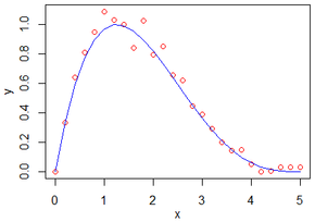
    Fruit growth rate modelling (Graph V. Letort - Le Chevalier, ECOLE CENTRALE PARIS)
      The blue line represents the 'true' model (a beta density function)
      The red dots stand for virtual measurements (simulated with an additive noise)

      The model is expressed as follow:

      BetaN formulae

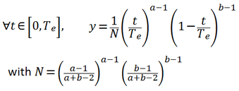
      The resulting data (17 measurements) are given below.
            x        y
        0.0     0.00
        0.3     0.48
        0.6     0.86
        0.9     0.99
        1.2     1.01
        1.5     0.91
        1.8     0.85
        2.1     0.77
        2.4     0.77
        2.7     0.41
        3.0     0.42
        3.3     0.22
        3.6     0.23
        3.9     0.02
        4.2     0.04
        4.5     0.00
        4.8     0.05

      Using the unweighted (Ω = Identity) least squares method, find estimates for the values of a and b.

      Enter the values found for a and b with one decimal and validate.
                a:           b:                    

        The following website can be used:
        http://statpages.org/nonlin.html .

        Indications using this online tool:
        - Enter the number of data points, variables and parameters
        In order to simplify the equations, translate both a and b values of one unit.
        - The function can thus be entered (copy and paste) as follows:
           Power(x/5,a) * Power(1-x/5,b) / ( Power((a/(a+b)),a)* Power((b/(a+b)),b) )
        - According to the distribution shape, initialize a and b values
        - Set the fractional adjustment factor to 0.2
        Copy the observed values and paste them in the Text Data Editor . Separate x and y values by a comma
        Click iterate button until reaching stable parameter values.
        Report the estimated parameter values.