GreenLab Course
Development
Stochastic axis branching modelling
-
At a given phytomer, the branching process is defined by three factors:
- its intensity, quantifying branching occurrence
- its delay, expressed in number of growth cycles, since branching can be immediate or delayed
- the branching pattern, not only as expressed in architectural botany, but also potentially showing couplings along the axis.
Branching intensity and delays
-
Branching intensity
-
Branching intensity, or in other words branching probability ai at a given
growth cycle N defines the probability of a new lateral axis occurring.
This value is in fact assigned to a physiological age couple (bearer physiological age and lateral axis physiological age) and classically retrieved from a simple ratio retrieved from distributions: branched phytomers out of total number of phytomers.
Branching delays
-
Branching may be immediate or delayed according to a specific delay law.
Note that F(i) the axis proportion waking up at growth cycle i, then the occurrences probabilities ai are roots of the following system:
- F(0) = a1 (probability of immediate branching)
F(1) = (1 - a1) . a2 (probability of branching in a second cycle, i.e. with a one cycle delay)
.....
F(i) = (∏k=1,i ( 1 - ak) ) . ai+1
Σk=0,iF(i) is the total number of phytomers branched at cycle i.
F can classically be adjusted to a sigmoid function (see previous chapter on mortality modelling).
Reversing the model, the branching probabilities can be computed from:

This formulation is generic:
- Immediate branching is defined by a1 = a, ai= 0 for all i > 1
Delayed crowns, corresponding to a constant delay d value, is sometimes observed in bushes. It can be defined by ad = a and ai = 0, for all i ≠ d

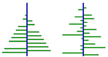
Simulating branching delays (Images P. de Reffye, CIRAD)
- Left: simulation of a constant branching delay of 7 growth cycles
Right: the same simulation with stochastic delays
Branching arrangements
-
Branching arrangements concerns several aspects related to relative branching positioning along a given axis.
According to botanical architectural branching patterns, branching may be continuous, diffuse or rhythmic.
Continuous or diffuse branching patterns can be simulated with the intensity model (with or without delays).
Rhythmic patterns can be shown on rhythmic growth, as branching positional patterns in growth units (acrotony, mesotony, basitony), usually with morphological gradients within the growth unit.
In such a case, one must first define the appropriate micro states and micro state sequences in order to mimic successive physiological age branching patterns (examples: growth units of poplar tree, pines, spruce, etc.).
However, branching rhythms on continuous growth, and within growth units, may also appear on phytomer sequences (simulated by the same micro-state). Such cases are classically studied using Markov Chains.
Remember that, in the GreenLab model, the fine geometrical position is not relevant, only the quantitative aspects for a given cycle and physiological age are; in practice a simple coupling model is efficient enough.
An example of simple branching coupling, with its estimation is given in the Application chapter ( ..\App\GLapp_fitst_017.html ).

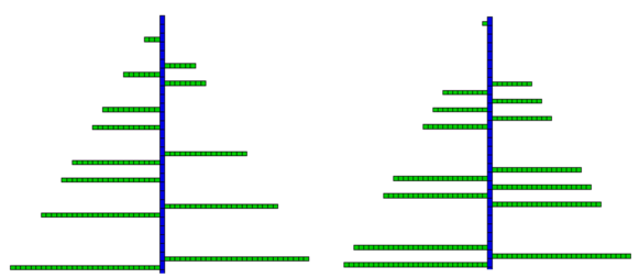
Simulating branching with coupling (Images P. de Reffye, CIRAD)
- Left: stochastic simulation with a branching intensity a = 0.5
Right: the same simulation with a coupling r = 0.7
