GreenLab Course
Development
Stochastic axis development modelling
-
We consider here the non-periodic random aspect of phytomer occurrence.
Modelling the development of axis
-
We associated a Bernoulli process of probability b of a new phytomer appearing.
Case of a constant occurrence probability
If probability b is constant during axis life, after N growth cycles, the distribution of the number of phytomers follows a Binomial Law B(N,b) (see preliminary Mathematical course).
The expected value of B(N,b), i.e. the average number of phytomers on the axis of N growth cycles is thus: M = N . b and the variance is V = N . b . (1 - b) = (1 - b). M
This simple model can thus be straightforwardly used on an axis showing continuous growth (cotton, coffee, etc.).
It is interesting to note that the relation between the expected value M and the variance V helps to define the b parameter from simple distribution measurements.
It only requires the computation of M and V for a significant number of axes, at different stages N of growth.
This is still true if the relation between the expected value and variance is not linear; such is the case of damped growth.
The case of damped growth
-
Let us suppose that the probability decreases along the axis according to:
b(i) = bi
it can thus be shown that, for a given growth cycle K, the expected value XN and the variance VN are respectively:
Once again, in this case, the definition of probability b can be derived from the relation between the expected value and variance, quadratic in this case.
This modelling approach is of great interest for practical use, since its full mean parameter (b) can be computed from statistics provided on phytomer distributions, resulting from actual plant internode counting.
This parameter fitting is described in the application chapter ( ../App/GLapp_fitst_012.html ).
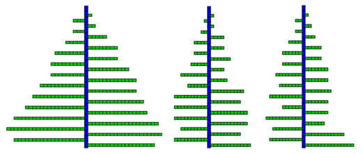
Of course, the rhythm ratio and Bernoulli process convolve, as shown below.

Binomial phytomer law distribution and rhythm ratio (Drawings P. de Reffye, CIRAD)
- Left: Physiological age 2 axis appears by a probability b = 0.8
Middle: The rhythm ratio of theses axis, in green, is now set to w2 = 0.5
Right: Another stochastic realization with b = 0.8 and w2 = 0.5
