COURSES

-> About this Resource
Scope *______
Map *____

-> Preliminary Courses
Contents & Objectives *__________________
Map *____
-> Botany
Contents & Objectives *__________________
Map *____
-> Axis Typology Patterns
Typology basis *___________
Pictograms *_________
Sexuality & development *___________________
Growth *______
Branching rhythms *______________
Branching delays *_____________
Branching positional *________________
Branching arrangement *__________________
Axis orientation *_____________
Architectural models *________________
-> Architectural Unit
About Arc. Models *______________
Models limitations *______________
Architectural Units *______________
Reiteration *_________
Sequence of development *___________________
Morphogenetic gradients *___________________
Physiological age *_____________
-> An Example
Wild Cherry (young) *_______________
Wild Cherry (adult) *______________
Wild Cherry (mature) *________________
Quiz *____
Case study Quiz *_____________
Supplementary resources *____________________

-> Eco-Physiology
Contents & Objectives *__________________
Map *____
-> Growth Factors
Factors affecting Growth *___________________
Endogenous Processes *_________________
Environmental Factors *_________________
Thermal Time *___________
-> Light interaction
P.A.R. *_____
Light absorption *_____________
Photosynthesis *___________
Respiration *_________
Maintenance respiration *__________________
L.U.E. Model *__________
Density effect *___________
Density effect on crop *__________________
-> Biomass
Biomass Pool *__________
Biomass Partitioning *_______________
Crop models *__________
A Crop model example *__________________
Quiz *____
Supplementary resources *___________________

-> Applied Mathematics
Contents & Objectives *__________________
Map *____
-> Probabilities
Section contents *____________
Discrete Random Variable *___________________
Expected value, Variance *___________________
Properties *________
-> Useful Laws
Bernoulli Trials *___________
Binomial Law *__________
Geometric Law *____________
Negative Binomial Law *_________________
-> Dynamic systems
Section contents *_____________
Useful functions *____________
Beta density *__________
Exercises *________
Negative Exponential *________________
Systems functions *______________
Discrete dynamic systems *___________________
Parameter Identification *__________________
Parameter estimation *________________
Supplementary Resources *____________________


-> GreenLab courses
GreenLab presentation *__________________
-> Overview
Presentation & Objectives *____________________
Map *____
Growth and components *___________________
Plant architecture *_______________
Biomass production *________________
Modelling - FSPM *______________
GreenLab principles *________________
Applications *__________
Supplementary resources *_____________________
-> Principles
Presentation & Objectives *____________________
Map *____
-> About modelling
Scientific disciplines *________________
Organs: tree components *___________________
Factors affecting growth *___________________
Model-simulation workflow *____________________
GreenLab inherits from *__________________
GreenLab positioning *_________________
The growth cycle *______________
Inside the growth cycle *___________________
Implementations *______________
Supplementary resources *____________________
-> Development
Presentation & Objectives *____________________
Map *____
Modelling Scheme *______________
Tree traversal modes *________________
-> Stochastic modelling
Principles *_______
-> Development
Growth Rhythm *____________
Damped growth *____________
Viability *______
Rhythmic axis *___________
Branching *________
Stochastic automaton *_________________
-> Organogenesis equations
Principles *_______
Organ cohorts *___________
Organ numbering *_____________
Substructure factorization *____________________
Stochastic case *____________
-> Structure construction
Construction modes *_______________
Construction basis *______________
Axis of development *________________
Stochastic reconstruction *___________________
Implicit construction *________________
Explicit construction *________________
3D construction *____________
Supplementary resources *____________________
-> Production-Expansion
Presentation & Objectives *____________________
Map *____
-> EcoPhysiology reminders
Relevant concepts *______________
Temperature *__________
Light interception *______________
Photosynthesis *___________
Biomass common pool *_________________
Density *______
-> Principals
Growth cycle *__________
Refining PbMs *___________
Organ cohorts *___________
GreenLab vs PbM & FSPM *___________________
-> GreenLab's equations
Summary *_______
Production equation *_______________
Plant demand *__________
Organ dimensions *______________
A dynamic system view *__________________
Equation terms *____________
Full Model *________
Model behaviour *______________
Supplementary resources *____________________
-> Applications
Presentation & Objectives *____________________
Map *____
-> Measurements
Agronomic traits *_____________
Mesurable/hidden param. *___________________
Fitting procedure *______________
-> Fitting structure
Principles *_______
-> Development
Simple development *_______________
Damped growth *____________
Rhythmic growth *_____________
Rhythmic growth samples *___________________
Mortality *_______
Branching *________
-> Crown analysis
Analysis principles *______________
Equations *________
Example / Exercise *_______________
-> Case study
Plant Architecture *______________
Development simulation *__________________
Introducing Biomass *_______________
Biomass partitioning *_______________
Equilibrium state *_____________
Supplementary resources *____________________

-> Tools (software)
Presentation & Objectives *_____________________
Map *____
Fitting, Stats *___________
Simulation *_________
Online tools *__________

GreenLab Course

Development

Stochastic axis viability modelling


A simple mortality case

    Mortality without development delays

      Let us first suppose that axis development shows no delays (rhythm ratio set to 1, and probability of phytomer occurrence for each cycle also set to 1, i.e. w = 1; b = 1.
      Let us then consider a distribution of living axes of K cycles, born from terminal buds whose survival probability - also called viability - is c.
      Then, the probability of staying alive in the next cycle is: cK+1, and thus the probability of becoming a dead branch is: (1 - c) . c K

      Mortality
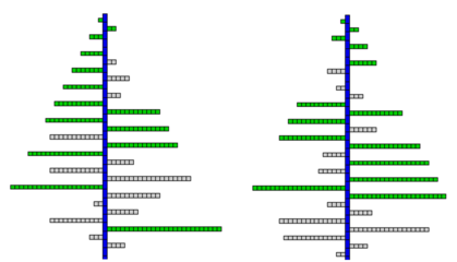
      Simulating terminal bud viability on a physiological age 2 axis (Images P. de Reffye, CIRAD)
        2 simulation examples with viability set to 0.95
        Dead axes are shown in grey
        Living axes are drawn in green

      The retrieval of viability c in this theoretical case can simply be assessed from the ratio of living and dead axes.


    Mortality with development delays

      Let us now consider the usual case with development delays where a new phytomer may appear according to a Bernoulli process with a probability b , and a viability c.
      The probabilities of staying alive or die at cycle K are unchanged, cK+1 and (1 - c) . c K respectively.
      This law is a truncated geometric distribution law, whose expected value MN and variance VN are respectively
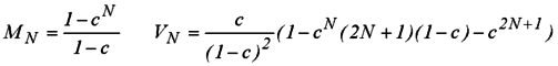
      Mean, variance geometrical law    (Eq. 1)

      However, the number of phytomers in a given axis of N cycles becomes complex, since the law is a composition of this geometric law and the binomial B(N,b) law.

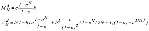
      The probability of an axis of N cycles having K phytomers is:

      Probability for an axis to have K phytomers

      The expected value and variance are then M = MN . d and V = b . (1 - b) . MN + b2 . VN with MN and VN as defined in (Eq. 1) giving finally:

      Mean and variance of axis length with N cycles


A generic mortality law

    We have seen that the death rate, or viability, when constant, can be retrieved from measurements on the living and dead axis statistics for given growth cycles.

    However, in many cases this viability rate is not stable with the age of the axis, i.e. with the number of cycles.

      In most cases, the mortality law is complex, following a sigmoid function shape.
      It is thus interesting to fit cumulated dead populations to a classic sigmoid function, leading thus to expressing meristem's viability along the axis as a function of the number of growth cycles, such that:

          S(i) = 1 - exp ( -α . iβ)

      Viability can then be expressed as:

          ci = exp ( -α . ( (i-1)β - (i-2)β ) )

      and the death rate at cycle i is given by:

          P(i) = exp ( -α . (i-1)β ) - exp ( -α . i β )

      See fitting page ( ../App/GLapp_fitst_016.html ) as an example.