COURSES

-> About this Resource
Scope *______
Map *____

-> Preliminary Courses
Contents & Objectives *__________________
Map *____
-> Botany
Contents & Objectives *__________________
Map *____
-> Axis Typology Patterns
Typology basis *___________
Pictograms *_________
Sexuality & development *___________________
Growth *______
Branching rhythms *______________
Branching delays *_____________
Branching positional *________________
Branching arrangement *__________________
Axis orientation *_____________
Architectural models *________________
-> Architectural Unit
About Arc. Models *______________
Models limitations *______________
Architectural Units *______________
Reiteration *_________
Sequence of development *___________________
Morphogenetic gradients *___________________
Physiological age *_____________
-> An Example
Wild Cherry (young) *_______________
Wild Cherry (adult) *______________
Wild Cherry (mature) *________________
Quiz *____
Case study Quiz *_____________
Supplementary resources *____________________

-> Eco-Physiology
Contents & Objectives *__________________
Map *____
-> Growth Factors
Factors affecting Growth *___________________
Endogenous Processes *_________________
Environmental Factors *_________________
Thermal Time *___________
-> Light interaction
P.A.R. *_____
Light absorption *_____________
Photosynthesis *___________
Respiration *_________
Maintenance respiration *__________________
L.U.E. Model *__________
Density effect *___________
Density effect on crop *__________________
-> Biomass
Biomass Pool *__________
Biomass Partitioning *_______________
Crop models *__________
A Crop model example *__________________
Quiz *____
Supplementary resources *___________________

-> Applied Mathematics
Contents & Objectives *__________________
Map *____
-> Probabilities
Section contents *____________
Discrete Random Variable *___________________
Expected value, Variance *___________________
Properties *________
-> Useful Laws
Bernoulli Trials *___________
Binomial Law *__________
Geometric Law *____________
Negative Binomial Law *_________________
-> Dynamic systems
Section contents *_____________
Useful functions *____________
Beta density *__________
Exercises *________
Negative Exponential *________________
Systems functions *______________
Discrete dynamic systems *___________________
Parameter Identification *__________________
Parameter estimation *________________
Supplementary Resources *____________________


-> GreenLab courses
GreenLab presentation *__________________
-> Overview
Presentation & Objectives *____________________
Map *____
Growth and components *___________________
Plant architecture *_______________
Biomass production *________________
Modelling - FSPM *______________
GreenLab principles *________________
Applications *__________
Supplementary resources *_____________________
-> Principles
Presentation & Objectives *____________________
Map *____
-> About modelling
Scientific disciplines *________________
Organs: tree components *___________________
Factors affecting growth *___________________
Model-simulation workflow *____________________
GreenLab inherits from *__________________
GreenLab positioning *_________________
The growth cycle *______________
Inside the growth cycle *___________________
Implementations *______________
Supplementary resources *____________________
-> Development
Presentation & Objectives *____________________
Map *____
Modelling Scheme *______________
Tree traversal modes *________________
-> Stochastic modelling
Principles *_______
-> Development
Growth Rhythm *____________
Damped growth *____________
Viability *______
Rhythmic axis *___________
Branching *________
Stochastic automaton *_________________
-> Organogenesis equations
Principles *_______
Organ cohorts *___________
Organ numbering *_____________
Substructure factorization *____________________
Stochastic case *____________
-> Structure construction
Construction modes *_______________
Construction basis *______________
Axis of development *________________
Stochastic reconstruction *___________________
Implicit construction *________________
Explicit construction *________________
3D construction *____________
Supplementary resources *____________________
-> Production-Expansion
Presentation & Objectives *____________________
Map *____
-> EcoPhysiology reminders
Relevant concepts *______________
Temperature *__________
Light interception *______________
Photosynthesis *___________
Biomass common pool *_________________
Density *______
-> Principals
Growth cycle *__________
Refining PbMs *___________
Organ cohorts *___________
GreenLab vs PbM & FSPM *___________________
-> GreenLab's equations
Summary *_______
Production equation *_______________
Plant demand *__________
Organ dimensions *______________
A dynamic system view *__________________
Equation terms *____________
Full Model *________
Model behaviour *______________
Supplementary resources *____________________
-> Applications
Presentation & Objectives *____________________
Map *____
-> Measurements
Agronomic traits *_____________
Mesurable/hidden param. *___________________
Fitting procedure *______________
-> Fitting structure
Principles *_______
-> Development
Simple development *_______________
Damped growth *____________
Rhythmic growth *_____________
Rhythmic growth samples *___________________
Mortality *_______
Branching *________
-> Crown analysis
Analysis principles *______________
Equations *________
Example / Exercise *_______________
-> Case study
Plant Architecture *______________
Development simulation *__________________
Introducing Biomass *_______________
Biomass partitioning *_______________
Equilibrium state *_____________
Supplementary resources *____________________

-> Tools (software)
Presentation & Objectives *_____________________
Map *____
Fitting, Stats *___________
Simulation *_________
Online tools *__________

Preliminary Course

Applied Mathematics

Probabilities. Discrete random Variables


Discrete Random Variable
    Formally, a random variable X is a measurable function from a probability space (Ω, F, P) to a measurable set (E,ε).

    More intuitively, let us consider chance experiments (or events) with a finite number or countable infinite number of possible outcomes.
    That is, the possible values might be listed, although the list might be infinite. The sample space Ω is the set of possible outcomes of the experiment.

    For example, we roll a dice and the possible outcomes are 1, 2, 3, 4, 5, and 6 corresponding to the side that turns up.

    A discrete random variable can then simply be considered as a function whose values correspond to the possible outcomes of a given chance experiment, possibly after some transformation is applied.

    For example, the outcome of the roll of one dice is a random variable X.
    And the sum of the outcomes of four independent dice rolls, Y = X1 + X1 + X2 + X3 + X4 , is also a random variable.
A famous historical example
    A dice game played an important historical role at the origins of the probability theory.

    Some famous letters between Pascal and Fermat were instigated by a request for help from a French nobleman and gambler, Chevalier de Méré.
    It is said that de Méré had been betting that, in four rolls of a die, at least one six would turn up.
    He was winning consistently and, to get more people to play, he changed the game to bet that, with a simple homothetic reasoning, in 24 rolls of two dice, a pair of sixes would turn up.
    However, the exact probability value is a bit more complicated than that: it is said that de Méré lost with 24 and, disappointed, considered that mathematics was wrong.

    In fact:
      1 - (5/6)4 = 0.5177... > 0.5
      1 - (35/36)24 = 0.4914... < 0.5
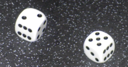

      Dices (Photo M. Jaeger, CIRAD)
Discrete Random Function
    The probability mass function p of a discrete random variable X satisfies the following properties:

      1. The probability that the random variable X can take a specific value j is p(j). That is:

        ∀ j ∈ Ω    P[X=j]  =  p(j) =  pj   ≥   0

      2. The sum of p(j) over all possible values of j is 1, that is
        Σj pj = 1
        where j represents all possible values that X can take.


      A consequence is that 0 ≤ pj ≤ 1