COURSES

-> About this Resource
Scope *______
Map *____

-> Preliminary Courses
Contents & Objectives *__________________
Map *____
-> Botany
Contents & Objectives *__________________
Map *____
-> Axis Typology Patterns
Typology basis *___________
Pictograms *_________
Sexuality & development *___________________
Growth *______
Branching rhythms *______________
Branching delays *_____________
Branching positional *________________
Branching arrangement *__________________
Axis orientation *_____________
Architectural models *________________
-> Architectural Unit
About Arc. Models *______________
Models limitations *______________
Architectural Units *______________
Reiteration *_________
Sequence of development *___________________
Morphogenetic gradients *___________________
Physiological age *_____________
-> An Example
Wild Cherry (young) *_______________
Wild Cherry (adult) *______________
Wild Cherry (mature) *________________
Quiz *____
Case study Quiz *_____________
Supplementary resources *____________________

-> Eco-Physiology
Contents & Objectives *__________________
Map *____
-> Growth Factors
Factors affecting Growth *___________________
Endogenous Processes *_________________
Environmental Factors *_________________
Thermal Time *___________
-> Light interaction
P.A.R. *_____
Light absorption *_____________
Photosynthesis *___________
Respiration *_________
Maintenance respiration *__________________
L.U.E. Model *__________
Density effect *___________
Density effect on crop *__________________
-> Biomass
Biomass Pool *__________
Biomass Partitioning *_______________
Crop models *__________
A Crop model example *__________________
Quiz *____
Supplementary resources *___________________

-> Applied Mathematics
Contents & Objectives *__________________
Map *____
-> Probabilities
Section contents *____________
Discrete Random Variable *___________________
Expected value, Variance *___________________
Properties *________
-> Useful Laws
Bernoulli Trials *___________
Binomial Law *__________
Geometric Law *____________
Negative Binomial Law *_________________
-> Dynamic systems
Section contents *_____________
Useful functions *____________
Beta density *__________
Exercises *________
Negative Exponential *________________
Systems functions *______________
Discrete dynamic systems *___________________
Parameter Identification *__________________
Parameter estimation *________________
Supplementary Resources *____________________


-> GreenLab courses
GreenLab presentation *__________________
-> Overview
Presentation & Objectives *____________________
Map *____
Growth and components *___________________
Plant architecture *_______________
Biomass production *________________
Modelling - FSPM *______________
GreenLab principles *________________
Applications *__________
Supplementary resources *_____________________
-> Principles
Presentation & Objectives *____________________
Map *____
-> About modelling
Scientific disciplines *________________
Organs: tree components *___________________
Factors affecting growth *___________________
Model-simulation workflow *____________________
GreenLab inherits from *__________________
GreenLab positioning *_________________
The growth cycle *______________
Inside the growth cycle *___________________
Implementations *______________
Supplementary resources *____________________
-> Development
Presentation & Objectives *____________________
Map *____
Modelling Scheme *______________
Tree traversal modes *________________
-> Stochastic modelling
Principles *_______
-> Development
Growth Rhythm *____________
Damped growth *____________
Viability *______
Rhythmic axis *___________
Branching *________
Stochastic automaton *_________________
-> Organogenesis equations
Principles *_______
Organ cohorts *___________
Organ numbering *_____________
Substructure factorization *____________________
Stochastic case *____________
-> Structure construction
Construction modes *_______________
Construction basis *______________
Axis of development *________________
Stochastic reconstruction *___________________
Implicit construction *________________
Explicit construction *________________
3D construction *____________
Supplementary resources *____________________
-> Production-Expansion
Presentation & Objectives *____________________
Map *____
-> EcoPhysiology reminders
Relevant concepts *______________
Temperature *__________
Light interception *______________
Photosynthesis *___________
Biomass common pool *_________________
Density *______
-> Principals
Growth cycle *__________
Refining PbMs *___________
Organ cohorts *___________
GreenLab vs PbM & FSPM *___________________
-> GreenLab's equations
Summary *_______
Production equation *_______________
Plant demand *__________
Organ dimensions *______________
A dynamic system view *__________________
Equation terms *____________
Full Model *________
Model behaviour *______________
Supplementary resources *____________________
-> Applications
Presentation & Objectives *____________________
Map *____
-> Measurements
Agronomic traits *_____________
Mesurable/hidden param. *___________________
Fitting procedure *______________
-> Fitting structure
Principles *_______
-> Development
Simple development *_______________
Damped growth *____________
Rhythmic growth *_____________
Rhythmic growth samples *___________________
Mortality *_______
Branching *________
-> Crown analysis
Analysis principles *______________
Equations *________
Example / Exercise *_______________
-> Case study
Plant Architecture *______________
Development simulation *__________________
Introducing Biomass *_______________
Biomass partitioning *_______________
Equilibrium state *_____________
Supplementary resources *____________________

-> Tools (software)
Presentation & Objectives *_____________________
Map *____
Fitting, Stats *___________
Simulation *_________
Online tools *__________

GreenLab Course

Development

Stochastic modelling implementation


Stochastic automaton

    Principles
      The dual-scale automaton can easily simulate stochastic transitions for both micro- and macro-scales.
      The principle is that each transition carries a probability of each process (development, mortality, branching) occurring.

      Be proceeding in this way, implementation respects the modelling principles, inspired from renewal theory.

    Continuous growth
      The Bernoulli process can be straightforwardly applied to micro-state (phytomers) transitions.
      And of course the rhythm ratio and the viability process too.

      In practice the rhythm ratio defines first whether or not a Bernoulli trial needs to be performed; then viability c is tested; if the terminal bud is still alive, development is finally tested (choosing a random number compared to the probability b).

      Applying the process growth cycle by growth cycle, the simulated axis can be encoded by single "1" and "0" codes, respectively standing for phytomer occurrence and rest.

    Rhythmic growth

      In theory, the same approach could be implemented for both micro- and macro-scales in the case of rhythmic growth.

      However, it is often more efficient to defined the production of the axis for the whole growth unit (the macro-state), and then distribute it (proportionally among micro-states).
      First, a random number K of phytomers is defined from the binomial law B(N,b), where N stands for the number of effective growth cycles (after a potential rhythm ratio filter).
      The corresponding macro-state thus holds K phytomers, with those mapped on the micro-state sequence defining the macro-state.

      The same approach applies to polycyclism, with pre-formed and neo-formed parts. In this case the K definition from the binomial law B(N,p) is replaced by Kp + Kn where Kp stands for the number of phytomers in the pre-formed part (also derived from a binomial law) and Kn stands for the number of phytomers in the neo-formed part (derived from a bionomial or a negative binomial law).

      As a result, the construction process leads to a similar output. The simulated axis is encoded by single "1" and "0" codes, respectively standing for phytomer occurrence and rest describing the growth unit sequence. Usually, according to their botanical definition, simulated growth units are separeted from each the other by rest sequences (list of "0").

    Branching

      Each micro-state may carry several whorls of lateral buds of different physiological ages.

      Each physiological age branching is tested, i.e. the delay expressed in the growth cycle is estimated.
      When coupling is modelled, branching simulation is potentially controlled by the branching results of the previous phytomer.
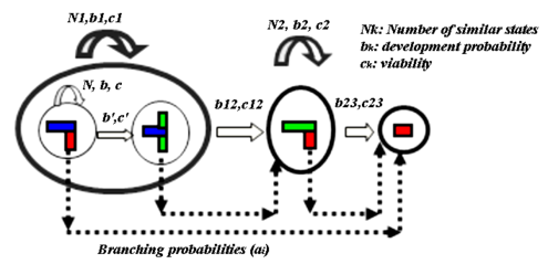
      Stochastic automaton
      Stochastic dual scale automaton (Images X. Xhao, Liama-CASIA and P. de Reffye, CIRAD)
        The dual scale automaton transitions are controlled by probabilities.
        At micro-scale level, transitions are controlled by the development and the viability probabilities
        b and c applied to the first micro-state sequence, while b', and c' apply to the first micro-state to second micro-state sequence.
        In the GreenLab model implementation those parameters are identical within macro-states (b=b' and c=c')
        Branching probabilities (including delays) are processed by the lower transitions (dotted arrows).


Stochastic sub-structures

    The use of sub-structures can also be extended to the stochastic case.

    Each deterministic substructure is replaced by a set of a limited number of sub-structures, as representative of the sub-structure distribution for the various phytomer typologies (in terms of expected value and variance).

    In a first step, the different sub-structure sets are built, starting from the older physiological ages to younger.
    At each branching, or physiological mutation, the sub-structures are chosen from ones already created.
    For practical reasons, the number of representatives is fixed at the same value, in order to minimize storage and construction costs.

      Stochastic sub-stuctures
      Simulating stochastic sub-structures (Images H.P. Yan, M.G. Kang, Liama-CASIA and P. de Reffye, CIRAD)
        In this example each sub-structure group has five stochastic representatives.
        Each representative is built using the higher sub-structure groups.
        Each sub-structure group shows appropriate statistical properties (the sample's expected value and variance fit the theoretical values)